Introduction

Niels Bohr was a very accomplished footballer and, specifically, a goal keeper. He played (alongside his brother) for one of the topic Danish teams – Akademisk Boldklub – situated near Copenhagen. Rumour has it that in one match he became distracted by a scientific problem he was mulling over and, whilst leaning against the goal-post to give it full thought, completely failed to respond to an opposition shot and conceded a goal! Who knows what the problem was, but it is fortunate he was so obsessed with maths and science because only a few years after the lapse in football concentration, Bohr was working with Ernest Rutherford at the University of Manchester and about to propose a major development to our understanding of atoms.

He was interested in the nuclear model of the atom recently described by Rutherford (see notes section 1.3), where a tiny nucleus was surrounded by orbiting electrons in empty space. In particular, he was concerned by a potential issue with this model. Bohr pointed out the problem in an article written in 1913, stating that while the Rutherford model accounted for the observed scattering of alpha particles by metal foils it didn’t seem to give a stable arrangement of electrons and nuclei. On the other hand, due to the different distribution of positive charge, the Thomson Plum Pudding model gave a more stable arrangement of electrons and nuclei, but wasn’t consistent with the alpha particle results.

Simply put, Bohr’s question was if the nucleus and electrons were thought of as charged particles why didn’t the electrons just spiral down towards the nucleus and get ever closer to it? This seems an obvious question and one that many A-level students often ask. After all, the nucleus is positively charged, the electrons are negative and we know that opposite charges attract one another.

This diagram shows my own interpretation of Bohr’s problem, with the dotted line showing the path an electron might take to the nucleus:

As Bohr pointed out, this couldn’t actually be happening, because if it was, we’d expect to observe atoms shrinking in size over time as the electrons collapsed inwards. In addition, calculations showed that large amounts of energy would be emitted by atoms even when they were in their normal states. However, there was no evidence for either of these things happening with real substances; atoms appear to have fixed sizes and the amount of energy you’d expect to be emitted by electrons spiralling in towards the nucleus far exceeds what is actually observed.

Linking atoms to quantum mechanics

Bohr decided that the answer to the problem involved combining Rutherford’s atomic model with the emerging concepts of “quantum mechanics”. These ideas were being developed by other prominent scientists of the time such as Max Planck and Albert Einstein and dealt with the behaviour of very tiny objects and particles, such as atoms and electrons. In quantum mechanics tiny particles behave in ways that seem incredibly odd to us in our “macroscopic” world where quantum effects go un-noticed at the much larger scales we are used to.

One of the strange properties of tiny particles like electrons is that they are restricted to having only a limited number of different energies- they cannot have any amount of energy at all, only specific values. To electrons energy is “quantised” which means fixed at different values. In our macroscopic world we don’t notice things like energy as being quantised and it seems to us as if we can change our energy to any value we want. For example, we can pedal ever so lightly faster or slower on a bike and apparently change our kinetic energy to any amount we want. But it isn’t that way for electrons; to them energy is quantised and they can only change from one specified value to another specified value by gaining or losing set amounts of energy.

Quantised energy levels in atoms

Bohr realised that he could explain how the Rutherford model was stable if he applied a quantum approach to atoms. He concluded that electrons within atoms were restricted to a limited number of specific allowed orbits with different energy, often referred to now as “energy levels”. Orbits closer to the nucleus were lower energy states, those further away had higher energy. However, any other positions around the nucleus were “forbidden” and electrons could not be in these positions. This alteration to the nuclear model removed the problem of electrons eventually closing in on the nucleus. A spiral in towards the nucleus would cover all the possible orbit distances and the existence of a fixed lowest-energy allowed state would always keep the electron some distance from the nucleus.

Tower block analogy

A common analogy that gives us an insight into the quantum world is to imagine the fixed electron energy levels as being like the floors inside a tall building. The building represents an atom and you are an electron. Within this building you cannot get to any height above the ground that you like, because you are limited to being on one of the different floors. These floor levels are fixed distances above the ground and you cannot change those – that’s just where the floors are. However, you can change your height above ground by going to one of the other floors, perhaps by using the lift. At a higher floor you effectively have more energy (gravitational potential energy in your case) as you are further from the ground.

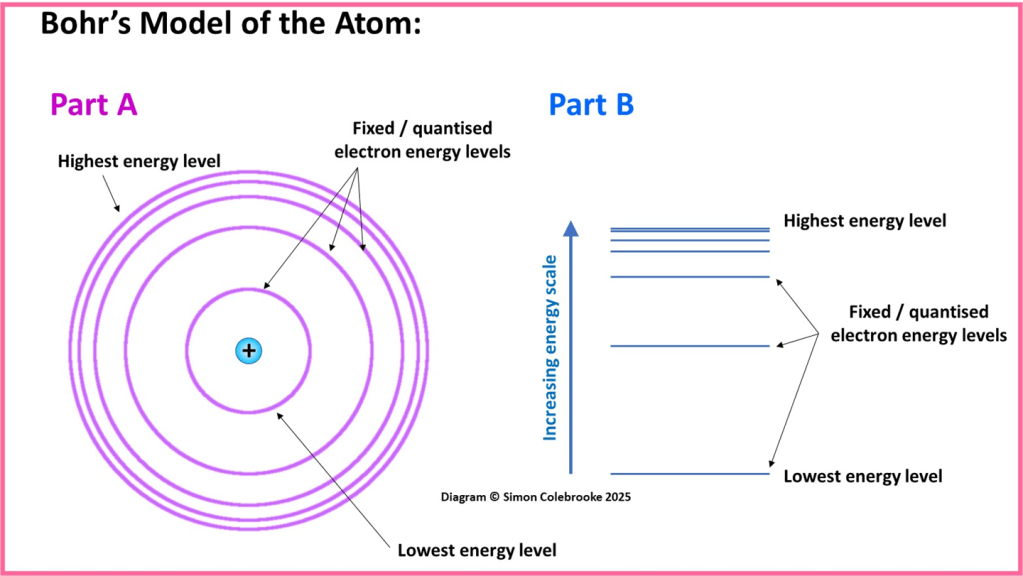
Bohr’s image of the atom is often shown using the two different representations below. Part A shows an atom with orbits at fixed distances from the nucleus, with higher energy orbits being further away. Part B shows the electron energy levels as horizontal lines indicating a position on a vertical energy scale, with increasing height corresponding to higher energy. The image in Part B is more useful and more commonly used at A-Level.

Key implications of Bohr’s ideas

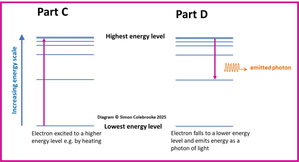
Bohr suggested that almost all of our experience involves atoms and molecules in their lowest energy states, with the electrons at the lowest energy levels (what exactly this means is quite complex and we will return to it many times in later sections). However, doing something to an atom which moves an electron to a higher energy state would result with the electron returning to the lowest level shortly afterwards and emitting a fixed amount of radiation when this occurred. A common example is a “flame test” where metal ions in a salt are put into a hot flame; heating the substance transfers electrons to higher energy levels and then, as they return to the lower levels, they emit energy in the form of light.

Part C of the diagram below shows what could happen to an electron as it was excited (moved) from a lower energy level to a higher energy level by heating. The pink arrow connects the start and end levels exactly as the electron energy is quantised and can only switch from one fixed level to another. The direction shows the electron movement. Part D shows the electron returning to the lower energy level and hence losing energy which is emitted as light.

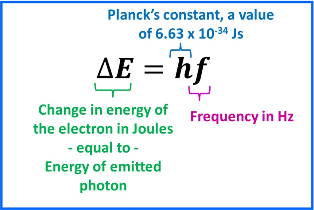
The emitted light could be thought of as a photon (note this is not a proton) which are packages or “quanta” of energy with a specific frequency. Different frequencies are interpreted by our eyes as different colours, hence the appearance of characteristic flames for different metal ions.

The energy change of the electron (the difference in energy between the initial and final energy levels) is equal to the energy of the emitted photon and related to the frequency by this equation:

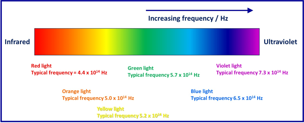
Hence larger electron energy changes correspond to a greater photon frequency. The visible portion of the electromagnetic spectrum and some approximate frequencies are shown below:

So, if an electron dropped from a high energy level to a lower level so that it’s energy changed by 3.78 x 10^-19 J, then the frequency of the emitted photon would be calculated like this:

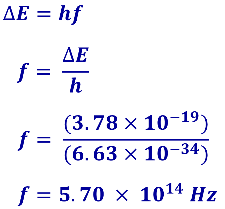
The calculated frequency is in the range expected for green light, so we’d observe a green colour for photons emitted in this process.

The emphasis of this section is on understanding the stages in development of atomic structure and the quantised nature of electron arrangements. However, much further details on photons and emission of light will be provided in the spectroscopy section and will be linked here when available.

Conclusion

Bohr found that he could use these new ideas to predict the energy levels of the electrons in a hydrogen atom and therefore the gaps in energy between the levels. This in turn allowed him to calculate the expected frequencies of light emitted by hydrogen atoms and accurately predict the appearance of the hydrogen emission spectrum. This was a convincing demonstration of the significance of his ideas and this aspect of atomic structure became increasingly important.

Although Bohr may not have saved quite as many goals as he could have done… he did contribute to saving the nuclear model of the atom (OK – I pushed it a bit with that analogy, but I think I got away with it alright!).

“Copyright Simon Colebrooke 14th April 2025”.

Suggested next pages

To read more about electron energy levels in atoms go to Section 1.9.

Alternatively, click the icons below to either return to the homepage, or try a set of questions on this topic (choose the Q icon) or return to the notes menu (N icon).

When writing this page I referred to the article by N. Bohr from 1913 entitled “On the Constitution of Atoms and Molecules” published in the Philosophical Magazine, 1913, 26, 1-25.

Update history:

Minor text changes and corrections 29^th June 2025.